When I first launched my Connections Eval (Aug 1st), Gemini 2.5 Pro was able to solve them with no sweat.
By August 7th, I had ran quite a few models on this could compare the results – including Gemini 2.5 Flash – which wasn’t so good at 9% solve rate (1 out of 11 puzzles).
A little bit after this, my buddy Pedram optimized the prompts for this and I landed version 2.0 (October 1st). The connections eval, as it exists today, has not changed prompts since this version. His optimization improved performance significantly for Gemini 2.5 Flash from 9% to 72% (more on this later).
When Gemini 3 Flash launched yesterday (December 17th, 2025), I figured I would test it out – you can see it in the results in the table above. 100% win pct, only 4 missed guesses. It was also roughly twice as fast: 27s per puzzle vs 54s, and half the cost. That is a very insane increase.
However, as I was evaluating the results, I discovered a flaw in my eval – there was too much variation in which puzzles were solved by which models. “No problem” I thought – because I knew there were some harder puzzles and I could evaluate which ones were the hardest and then give only the hardest puzzles to my models. No problem, right?
Perhaps not. I gave Gemini 3 Flash every puzzle 10 times and it solved every single one, while sipping tokens, and ran 410 puzzles in 22m52s. Total cost: $3.03.
My eval is dead, and Gemini 3 Flash killed it.
So how far have we came since Gemini 2.5 Flash? Now that I have a nice test harness for ranking puzzles, lets run it for the older Gemini Model.
Run time: 1h7m37s. Cost: $8.30. Accuracy? 60%. Incredibly progress by the Gemini team in just 6 months.
So whats next? I’m working on my BASED eval – which has a head-to-head games of Codenames for my set of evals. I suspect it will be much harder to for the models to saturate this one!
I’ve been spending time doing some work with AI – and this blog is just a “check-in” journal on what has been working for me.
This blog will begin with “Idea Honing” (mini PRD) and then move to an iterative development workflow, followed by an example project.
Idea Honing
You need to spend some time honing your idea. There is a great blog on this subject which contains a great prompt to help step through your idea.
Ask me one question at a time so we can develop a thorough, step-by-step spec for this idea. Each question should build on my previous answers, and our end goal is to have a detailed specification I can hand off to a developer. Let’s do this iteratively and dig into every relevant detail. Remember, only one question at a time.

Here’s the idea:

<IDEA>
You should use the best LLM available to you for this, as you want clarity of words & thought. As of this writing (Sept 1st 2025), Gpt5 & Gemini 2.5 Pro work great for this. I also maintain a leaderboard for wordcel evals – using any of the top models should work great.
One tweak I have added to Harper’s blog is the last step, where he suggests to wrap up – make sure to add “Give me the final output as XML” – for whatever reason this works great!
Development Environment
Lately I have been using vanilla VS Code + Amp. It’s pretty simple to install the plugin and get started – but this is a paid tool! I find I spend somewhere around $5/hr when I use it, which seems fine in the context of my other hobbies.
What’s great about having an environment this simple is that it works great on Windows, Mac, & Linux, so I can seamlessly switch between them based on how I work.
Once you have the environment set up (should take you like 5 minutes or less), you can get started with prompt. Create a new folder for your project, open VS Code, and pass the prompt from the previous step into Amp.
Other Helpful Environment Add-ons
There are ton of niche tools you can add to your environment, so I am simply going to call out the ones I use regularly.
These three tools (frameworks? libraries?) will get you very far.
Interacting with your LLM while coding
If you have a simple idea and a good prompt, most of the time your LLM can “one-shot” it by getting you a working prototype with a single prompt. Your goal when building this stuff should always be to decompose your problem into individual, runnable steps, like the Agile car analogy of yore. This is particularly important with LLMs as every time you can run the program, you can also test it. This is critical because you want to keep these steps small so you can commit your changes into source control once whatever your current set of tests is, passes. Then you can give the LLM a new prompt to continue forward from a stable base.
Once I get the first runnable prototype, I do my first commit and spin up the repo in Github. Make sure to do this! LLMs are not deterministic and can destroy your project at any time, as has been memed numerous times on twitter (and a few weeks later, LinkedIn).
Testing
There are a couple of ways that seem to work well for LLMs with testing. I will outline two approaches.
Option 1: Just use the software
This is my typical approach. I just use the thing and modify it as I see fit, and fix bugs as I go. Once it works like I want it to, only then do I add tests – basically to make sure that future changes do not break existing functionality. Of course, LLMs are great at adding tests!
Option 2: Test Driven Development (TDD)
For more complex codebases, it seems like TDD is the way to go. I find it to be overkill for the hobby project but you can indeed write all your tests first and then let the LLM “solve” the tests. For complex logic puzzles (i.e. NFL tiebreaker logic), TDD is a much better approach than brute force by using the software and fixing bugs as they come up.
A practical example
I did a small project over labor day weekend to create a chrome extension to copy a screenshot and turn it into a csv. The below part will be very long because it is going contain the full idea honing transcript and prompt.
Initial Idea Honing Transcript
User: Ask me one question at a time so we can develop a thorough, step-by-step spec for this idea. Each question should build on my previous answers, and our end goal is to have a detailed specification I can hand off to a developer. Let’s do this iteratively and dig into every relevant detail. Remember, only one question at a time.
Here’s the idea: a chrome extension called “csv everything” that lets you take a screenshot and turn it into a csv, which is downloaded by your browser. behind the scenes it makes an API call (using your own API key) to open router with the image, then returns the result as csv. If it cannot identify if its a table, it should tell the user “couldn’t translate to csv”. It should also work with charts – basically it will give you the data points that allow you to build a line / bar / scatter chart.
Gemini: Of course. This is a great way to build a detailed spec. Let’s start with the user’s first action.
After the user installs the extension, how do they initiate the screen capture? For example, do they click the extension icon in the toolbar, which then allows them to drag and select an area on the page?
User: initially it takes whatever is in clipboard, verifies if it is an image, and if so, uses it. If its not an image, it tells the user “copy an an image of the data first”
Gemini: Got it. The trigger is clicking the extension icon, which then checks the clipboard.
Now, let’s think about the necessary credentials. The extension needs the user’s OpenRouter API key to make the API call.
Where and when does the user input and save their API key? For instance, is there a settings page, or does a field pop up the very first time they use the extension?
User: in the extension settings
Gemini: Excellent, a standard settings page is a clear approach.
Let’s refine the user flow for someone who is just getting started. A new user installs the extension, copies an image of a table, and clicks the extension icon, but they haven’t entered their API key in the settings yet
What should the extension do at this point? For example, should it show a message like “API key not found, please add it in settings” with a button that takes them there?
User: it show a message like “API key not found, please add it in settings” with a button that takes them there
Gemini: Perfect, that’s a very user-friendly flow.
Now, let’s move to the core action. The extension has the image from the clipboard and the user’s API key. It’s ready to make the call to the OpenRouter API.
What specific instructions (i.e., the prompt) should the extension send along with the image? For example, should it be a simple instruction like, “Extract the data from this image into CSV format, including headers if present”?
User: we can hone the prompt later as part of the testing. but yes, for now lets use a place holder “turn the image into a csv”. maybe the user can tune the prompt in their settings?
Gemini: Excellent idea. Making the prompt customizable in the settings is a powerful feature for advanced users. We’ll add that to the spec for the settings page.
So, the API call has been sent with the image and the user-defined prompt. This process might take a few seconds.
What should the user see in the extension’s interface while it is actively processing the image and waiting for a response from the API? For example, should it display a loading animation or a message like “Generating your CSV…”?
User: it should have a little spinner like the download icon in chrome – a dotted line spins around the outside of the icon.
Gemini: Got it, a spinner animation that mimics the native Chrome download icon will provide clear visual feedback.
Now, let’s handle the two possible outcomes of the API call. We’ll start with the successful one
The spinner stops, and the extension has received valid CSV data from the API. What should happen next? Should it automatically trigger the browser’s download functionality for the `.csv` file? And what should the default filename be?
User: “data.csv” is the default name, it should trigger the “save file” pop over
Gemini: Understood. The extension will trigger the standard “Save As” browser dialog, pre-filling the filename as `data.csv`.
Now, let’s cover the other scenario. The API call finishes, but the model could not interpret the image as a table or chart.
What exactly should the extension show the user in this case? For example, does the popup window display the text “couldn’t translate to csv” with a “Try Again” button?
User: it needs to identify error state – if there is an issue with the API call (anything other than 200) it should tell the user the specific error. if the image failed to turn into the chart but the API call succeeded, it should say “could not convert this image to a csv” – I think the challenge here is that “try again” implies that the image could be converted to a csv but in many cases it probably cannot be, because users are pasting in bad images.
Gemini: That’s an excellent distinction between an API error and a conversion failure. We will add that specific logic to the spec.
So, when the popup displays either an API error (like a 401 or 500) or the “Could not convert this image to a csv” message, how does the user dismiss it to end the current attempt? Should there be a simple “OK” button, or can they just click away from the popup to close it?
User: Yeah just hit an “X” in the corner. “OK” doesn’t do anything for the user in this case, so its more an FYI
Gemini: Perfect, an “X” to close notifications is clean and simple.
Now, let’s circle back to a key feature you mentioned in the original idea: processing charts. So far, the logic we’ve built is perfect for images of tables.
Does this same process and prompt—”turn the image into a csv”—also apply to images of line charts, bar charts, or scatter plots? Or does the extension need to handle charts differently in some way?
User: yes, the prompt should be the same. if the user wants a more sepcific prompt, they can tune in the settings
Gemini: Excellent, that simplifies the core logic. The extension will use the same process for all images and rely on the model’s intelligence and the user’s custom prompt for specific needs.
We have now defined the entire end-to-end user flow. Let’s refine one last detail on the settings.
OpenRouter provides access to many different AI models (like GPT-4o, Claude 3, etc.), which have varying costs and performance. Should the extension use a single, hard-coded model for all users, or should there be a dropdown menu in the settings page allowing the user to choose which model they want to use?
User: it should be set by default to gemini 2.5 pro, but allow the user to pass a model string from open router if they want.
Gemini: Got it. We’ll set a sensible default model but give the user full control to override it. That’s a perfect balance.
I believe we have now covered the entire specification from the first click to the final output, including settings and error handling. I will now compile everything into a final summary that you can hand off
Editor’s Note: Removed the plain text spec for brevity, as its included in XML below
This completes the specification. Does this detailed summary accurately reflect your vision for the extension?
User: give me this spec a xml please
Gemini: Of course. Here is the complete specification formatted as XML.
<?xml version="1.0" encoding="UTF-8"?>
<specification project="csv everything">
    <description>A Chrome Extension to convert images of tables or charts into a downloadable CSV file using the OpenRouter API.</description>

    <coreFunctionality>
        <trigger>User clicks the extension icon in the Chrome toolbar.</trigger>
        <inputSource>
            <source>Image from the user's clipboard.</source>
            <logic>
                <case condition="Image found">The process begins.</case>
                <case condition="Image not found">An error is shown (see Error Handling).</case>
            </logic>
        </inputSource>
        <processing>
            <api>OpenRouter</api>
            <details>The extension sends the clipboard image and a prompt to the API using the user's configured credentials.</details>
        </processing>
        <successfulOutput>
            <action>Triggers the browser's native "Save As" dialog.</action>
            <defaultFilename>data.csv</defaultFilename>
        </successfulOutput>
    </coreFunctionality>

    <userInterface>
        <state type="in-progress">
            <indicator>A loading spinner that visually mimics Chrome's native download icon.</indicator>
            <description>Displayed in the extension popup while waiting for the API response.</description>
        </state>
        <state type="notification">
            <dismissal>User clicks an "X" icon in the corner of the message box.</dismissal>
            <description>Applies to all error and informational messages.</description>
        </state>
    </userInterface>

    <settingsPage>
        <description>A standard options page for user configuration.</description>
        <fields>
            <field name="OpenRouter API Key">
                <type>Text Input</type>
                <required>true</required>
                <purpose>To securely store the user's API key.</purpose>
            </field>
            <field name="Model String">
                <type>Text Input</type>
                <required>false</required>
                <purpose>Allows the user to specify which OpenRouter model to use.</purpose>
                <defaultValue>google/gemini-2.5-pro</defaultValue>
            </field>
            <field name="Custom Prompt">
                <type>Text Area</type>
                <required>false</required>
                <purpose>Allows the user to define the prompt sent to the model. Used for all image types (tables, charts, etc.).</purpose>
                <defaultValue>turn the image into a csv</defaultValue>
            </field>
        </fields>
    </settingsPage>

    <errorHandling>
        <case condition="No Image in Clipboard">
            <message>Copy an image of the data first</message>
        </case>
        <case condition="Missing API Key">
            <message>API key not found, please add it in settings</message>
            <action>Provide a button that directs the user to the settings page.</action>
        </case>
        <case condition="API Call Failure">
            <trigger>API responds with a non-200 status code (e.g., 401, 500).</trigger>
            <message>Display the specific error returned by the API.</message>
        </case>
        <case condition="Conversion Failure">
            <trigger>API responds with a 200 status code, but the model could not extract data.</trigger>
            <message>Could not convert this image to a csv</message>
        </case>
    </errorHandling>

</specification>
From here I took that spec into an empty directory with VS Code and Amp, and they took it from there. I did end up modifying it so you could run it in the background, but otherwise the initial spec was bang on. You can take a look at the repo here: CSV Everything.
Interactions with AmpCode
The interactions with Amp once I had the spec were fairly trivial. Here are my iterative prompts with Amp, after the initial spec. My specific prompts are always in quotes and my commentary is unquoted, as such you will see some typos in my prompt.
“Next we need to build and test. how do i package it so i can load it in my chrome for testing?” (Once I had this answer, I immediately began testing this locally, and all the questions below all follow that line of thought)
I noticed it was building an icon in png, so I interrupted and said “Lets use SVG just so we can test”
“change the icon to be the text “CSV””
“in my testing, the response from gemini comes in markdown ““`csv <text> “` the markdown formatting shouldn’t be passed to the csv file that is created, so please strip that away. Also, the icon isn’t loading. I think we do need to render the png.”
I noticed it was using the system python to generate an icon so I stopped it and said “use uv instead”
“lets change the Icon to be bold, black text on a transparent background.”
“Ok, so when I click off the extension or change tabs, the api call is interuptted. Is there a way to make it run in the background once the conversion is started?”
“when its running, is there any way in indicate the extension icon is doing something to the user? like a little blue dot or something”
“I tried to use Gemini Flash, and it failed. Is that because 2.5 pro is a reasoning model and Flash is not?”
“Hmm, I’m not getting good enough error messages. Pro works, but flash doesn’t. I can see the API calls making their way to open router, but the response isn’t coming showing up. We should log the entire response from openrouter when we are in “debug mode”, which is a flag in the settings (enable debug mode : true/false), even if it is invalid.”
“seeing this error: Background conversion error: TypeError: URL.createObjectURL is not a function” (note: I also included a screenshot of the error)
“ok the indicator for when its running is way too big. It should a small blue dot in the top right of the icon area. 1/4 the size of current indicator.”
“change the text to a “down arrow””
“Ok so i am working on publishing to Chrome, and it is asking me why i need the “Host Permission” – can we rework this to work without that permission? If not, why?”
And here is a couple of demos!
Conclusion
As you can see you, it is fairly simple to get started with these tools but there is a lot of depth in How you use them. I hope this is helpful glance into the current state of how I am using them and that you find this type of journaling useful.
A few months ago, Benn Stancil wrote about the eternal spreadsheet. While I appreciated the generous shout out to both mdsinabox and motherduck (my employer), this really got the wheels turning around something that I have been feeling but have only been able to put into words recently: are BI tools transitory?
Consider the following scenario in the Microsoft stack: ingest data with ADF, transform with Fabric (& maybe dbt?), build a semantic model in Power BI, and delicately craft an artisanal dashboard (with your mouse). Then your stakeholder takes a look at your dashboard, navigates to the top left corner and clicks “Analyze In Excel”. How did we get here?
I remember back in the 90s, hearing my dad talk about “killer apps”. The killer app was the app that made your whole platform work. If you wanted your platform to be adopted, it needed a killer app so good that users would switch their hardware and software (an expensive proposition at the time) so they could use the killer app. In my lifetime, I recall a few killer apps: The App Store (iOS), the web (Internet), and Spreadsheets (personal computing).
Spreadsheets allowed a user to make an update in one place and for the data to flow to another place. If this concept seems oddly like a directed-acyclic graph (DAG), that’s because it is. These spreadsheets contain a bunch of features that we find handy in the data solutions stack today: snapshots (save as), version control (file naming), sharing (network shares & email attachments), business intelligence (pivot tables & charts), file interoperability (reading csv, json, xml etc), transformation (power query (there was an earlier, even more cursed version too)). All of these pieces have obvious metaphors in the commonly used data stacks today. Critically, one piece is missing: orchestration (note: back in mid 2010s, I used and loved an excel plugin called “Jet Reports” that included an orchestrator, among other things). Now if you were running a business in the 90s (like these guys), there was no need for orchestration in your spreadsheet. You, the business user, were the orchestrator. Your data came from many places – memos (later, emails), research (books, later pdfs), a filing cabinet (later, databases), phone calls (later, slack), meetings (later, zoom calls), and your own synthesis (later, chatGPT (just kidding)). Software could not contain these! We did not have the digital twins for these analog processes. In some ways, the spreadsheet was the perfect digital collection point for these physical artifacts.
As each of these parts of our business decision making input processes transitioned to digital, our poor spreadsheet began to fall out of favor. We replaced memos with emails, phone calls with IM (via skype, if you are old enough to remember), and so on. And these digital processes began to produce loads of data. Every step produced an event that was stored in a database. The pace of change in the business environment increased in-kind. Our once per month spreadsheets orchestrated by humans were a bit too slow, processes produced too much data to be aggregated by humans. I fondly recall the launch of excel 2007, which included a new architecture and file format, so that we could process one million rows instead of only 65,536.
Unfortunately, the hardware at the time could not actually handle one million rows. Every single person using excel, unencumbered by 32bit row limits, ran into the hard limits of the Excel architecture and inevitably seeing a spinning, “waiting for excel” icon before crashing (hopefully you saved recently). Hilariously, Microsoft trained users to tolerate an absolutely terrible experience. Excel could do too much. What we needed to do was unbundle this tool, take it apart piece-by-piece, so that we could have good, delightful experiences for our business users. Users could still use spreadsheets for things, but we needed to shift the load bearing intelligence of our business decision making into better tools.
So we built even more powerful databases, and ways to automate decision making at scale. We began to use multiple computers, running in parallel, to solve these problems for us. Large complex systems like Hadoop were required to aggregate all this data. Companies like Google harnessed the immense scale enabled by these systems to become the largest in the world, building never-before-seen products and experiences.
At the same time, CPU clock speeds stopped increasing. We had maxed the number of cycles we could push out of the silicon in the fabs. But innovation found a way to continue – we began to add more cores. Slowly but surely Moore’s law kept on holding, not on clock speed but on throughput.
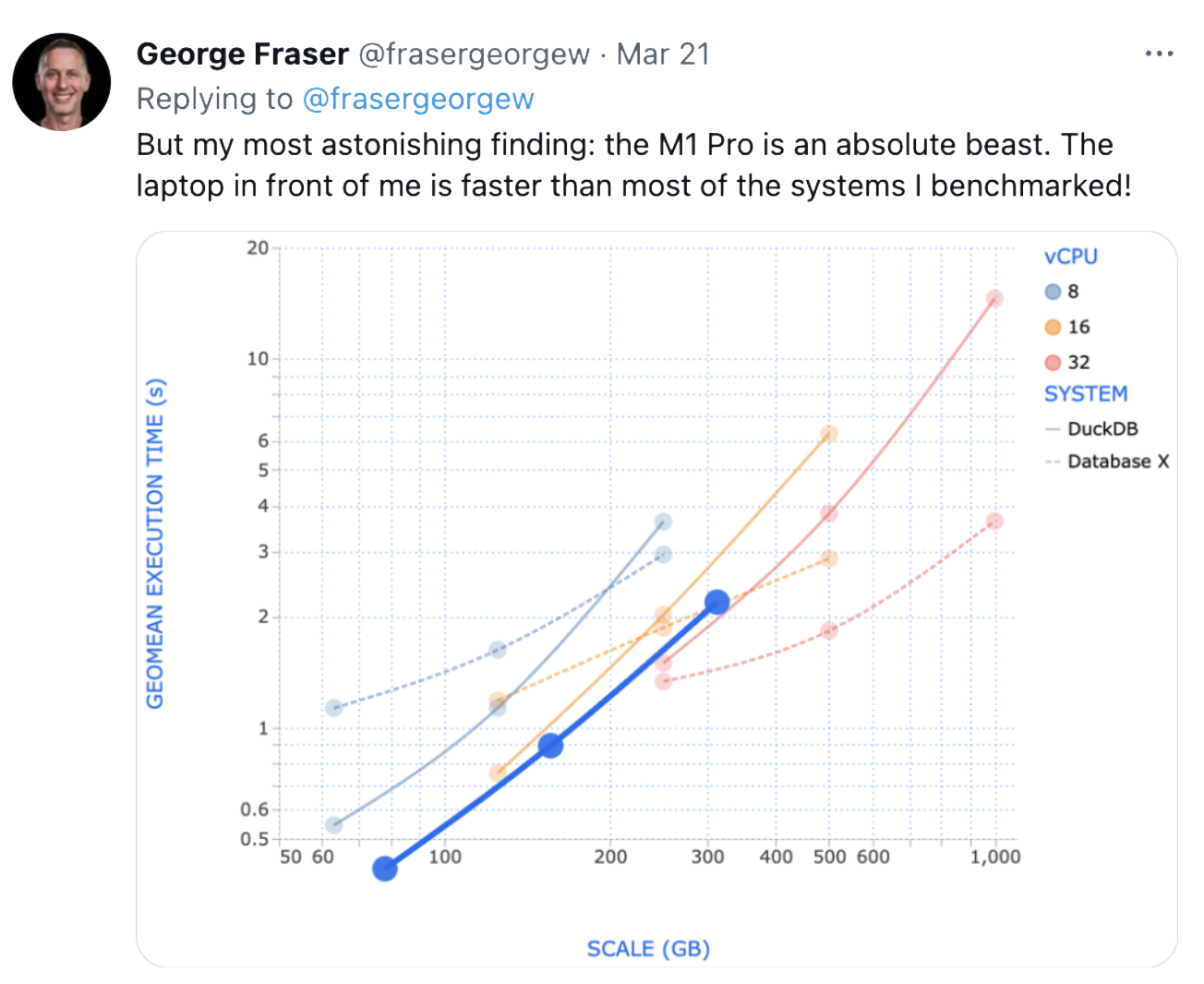
The software built to take advantage of the scale that was possible with huge quantities of networked computers made assumptions about how to work at great scale across many machines (i.e. Spark). These assumptions did not generalize to single machines with many cores. This has not been unnoticed, of course (see George’s tweet).
So what happened to our business intelligence while this was going on? The number of tools exploded, while the consumption interface remained unchanged. Categories were split into sub-categories into sub-categories. We only had so many charting primitives, and whether we dragged and dropped with Tableau or used BI as code in Evidence, the output looked largely the same. But instead of one tool that we needed in the 90s, we now had thousands.
But I would argue we haven’t added anything new, we’ve merely unbundled it into a bunch of different products and that don’t work that great together. REST APIs have allowed scalable, loosely coupled systems but really suck to work with. Behind every large enterprise data workflow is an SFTP server with CSVs sitting on it (if you are lucky, its object storage and a compressed format, but its the same thing).
If we look at the trends, in 5 years we will have approx. 10x more compute than we do today, and Backblaze estimates that cost per GB of storage will stabilize around 0.01 / GB ($10/TB). If these trends hold, we will easily have enough horsepower on our laptops to put all these pieces that we have decoupled over time, into one box. If BI tools are transitory, spreadsheets are eternal. The era of spreadsheets 2.0 will be upon us.
What are the characteristics of Spreadsheets 2.0?
Runs on a single node with many cores (hundreds?)
One file format for handling all types of data (xlsx++)
One language for end-to-end data manipulation (sql)
A spreadsheet UI for interacting with data at any step in the data manipulation (power query-ish)
An AI trained on all these parts above to assist the user in documentation, understanding, and building (clippy but good)
I believe the first building block of this has emerged in front of our eyes: DuckDB. The hardware is being built as we speak (the feedback loop will build it whether we like it or not). Julian Hyde is advocating for “completing the SQL spec to handle metrics” (with apologies to Malloy) – humans have refined this language over the last 50 years and will continue to do it for the next 50. We already have the UI primitives (Excel), so we merely need to bolt these together.
It’s time for the humble spreadsheet to RETVRN. It’s time to bring humans back into the workflow, empowered by AI, to own the data ingestion, transformation, and synthesis required to make decisions. Of course, I’m tinkering with this idea today, if you are interested in what I have so far, please reach out, I would love to talk.
AI-powered tools are transforming the way we code, and I recently got a chance to dive into this revolution with Codeium’s Windsurf IDE. My journey spanned two exciting projects: updating the theme of my mdsinabox.com project and building a Terraform provider for MotherDuck. Each project offered unique insights into the capabilities and limitations of AI-enhanced development. It should be noted that I did pay for the “Pro Plan” as you get rate limited really quickly on the free tier.
My first project involved updating the theme of my evidence.dev project. Evidence.dev is a Svelte-based app that integrates DuckDB and charting (via ECharts). Styling it involves navigating between CSS, Svelte, TypeScript, and SQL—a perfect storm of complexity that seemed tailor-made for Windsurf’s AI workflows.
I aimed to update the theme fonts to use serif fonts for certain elements and sans-serif fonts for others. Initially, I asked the editor to update these fonts, but it failed to detect that the font settings were managed through Tailwind CSS—a fact I didn’t know either at the time. We wasted considerable time searching for where to set the fonts.
the windsurf editor using cascade (right pane) to update the code
After a frustrating period of trial and error of pouring over project internals, and later reading documentation, I realized that Tailwind CSS controlled the fonts. Once I instructed the editor about Tailwind, it identified the necessary changes immediately, and we were back on track.
updated theme on the nba team pages
However, one gripe remained: Windsurf’s model didn’t include the build files for the Evidence static site, so I had to manually copy files to another directory for it to work. Additionally, debugging errors using the browser’s source view proved more efficient than relying on the editor. These limitations were a bit frustrating, but the experience highlighted the importance of understanding your project’s architecture and guiding AI tools appropriately. Access to a browser emulator would massively improve the debugging experience.
Project 2: Building a Terraform Provider for MotherDuck
The second project was sparked by a potential customer’s request for a Terraform provider for MotherDuck. While I was familiar with Terraform conceptually, I’d never used it before. With the recent launch of our REST API at MotherDuck, this felt like the perfect opportunity to explore its capabilities.
I instructed Windsurf, “I want to make a Terraform provider. Use the API docs at this URL to create it.” The editor sprang into action, setting up the environment and framing the provider. While its initial implementation of the REST API was overly generic and didn’t work, the tool’s ability to see the entire codebase end-to-end made it relatively straightforward to refine. I did have to interject and say “here is an example curl request that I know works, make it work like this” which was enough to get it unstuck.
intervening with cascade to tell it to change directory instead of run go init (again)
As an aside, observing it at times was quite comical as it seemed to take approaches that were obvious incorrect, especially when I was dealing with some invalid authorization tokens. It would almost say “well I trust that my handler has given me a valid token, so it must be something else” and just start doing things that were obviously not going to work.
Anyway, once the main Terraform file was built, I tasked the editor with writing tests to validate its functionality. It recommended Go, a language I had no prior experience with, and even set up the environment for it. Through a mix of trial and error and manual intervention (particularly to address SQL syntax issues like the invalid ‘attach if not exists’ statement in MotherDuck), I managed to get everything working. From start to finish, including testing, the entire process took around four hours—which seemed pretty decent given my experience level.
Conclusion
My experience with Codeium’s Windsurf IDE revealed both the promise and the current limitations of AI-enhanced development. The ability to seamlessly navigate between languages and frameworks, quickly scaffold projects, and even tackle unfamiliar domains like Go was incredibly empowering. However, there were moments of friction—misunderstandings about project architecture, limitations in accessing build files, and occasional struggles with syntax. Getting these models into the right context quickly is pretty difficult with projects that have lots of dependencies and overall my projects are fairly low complexity.
Still, it’s remarkable how far we’ve come. AI-enabled editors like Windsurf are not just tools but collaborative partners, accelerating development and enabling us to take on challenges that might have otherwise seemed impossible. As these technologies continue to mature, I can’t wait to see how I can use them to build even more fun projects.
Over the weekend I spent some time getting uv running on mdsinabox.com to see what the hubbub was about. As it turns out, it was harder than expected because of permission issues inside of dev containers & github actions.
The existing documentation on the uv github repo as well as docker instructions from ryxcommar’s blog are not pointed at my scenario, which is running it in a docker image and in CI. This blog post is up so if others run into this issue, they can find it and add it to their set up as well.
How to run uv in a dev container
Since we are using system python with uv, we need to tweak some settings in our dev container. There are two changes to make: (1) run as root user, and (2) add ““chmod 777 /tmp to your postCreateCommand. In your devcontainer.json, add or modify the following lines:
Then you can run `uv pip install --system -r requirements.txt in your devcontainer to add libraries as needed.
How to run uv in Github Actions
Now that we are using system python in our dev container, we also need to add one step to get the perms setup in CI. And that step is to add a python setup step in the Github action before running uv.
...
    steps:
      - name: Set up Python
        uses: actions/setup-python@v2
        with:
          python-version: '3.11'
...
Using the “actions/setup-python@v2” github action step will set up your runtime environment to properly interact with `uv pip install --system. Shout out to Charlie, of course, who very helpfully PR’d this into the mdsinabox repo.
Hope you find this useful! Please feel free to drop me a line on twitter @matsonj if you have any comments or feedback.
The variant of “Super Bowl Squares” that we analyzed is one in which the entrant is assigned a digit (0-9) for Team A’s final score to end with and a digit for Team B’s final score to end with 1
We compiled the final game scores from the 30 most recent NFL seasons to determine the frequency that each of the 100 potential “Squares” has been scored a winner
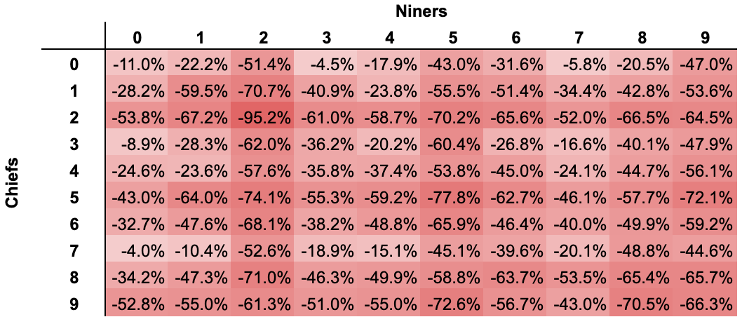
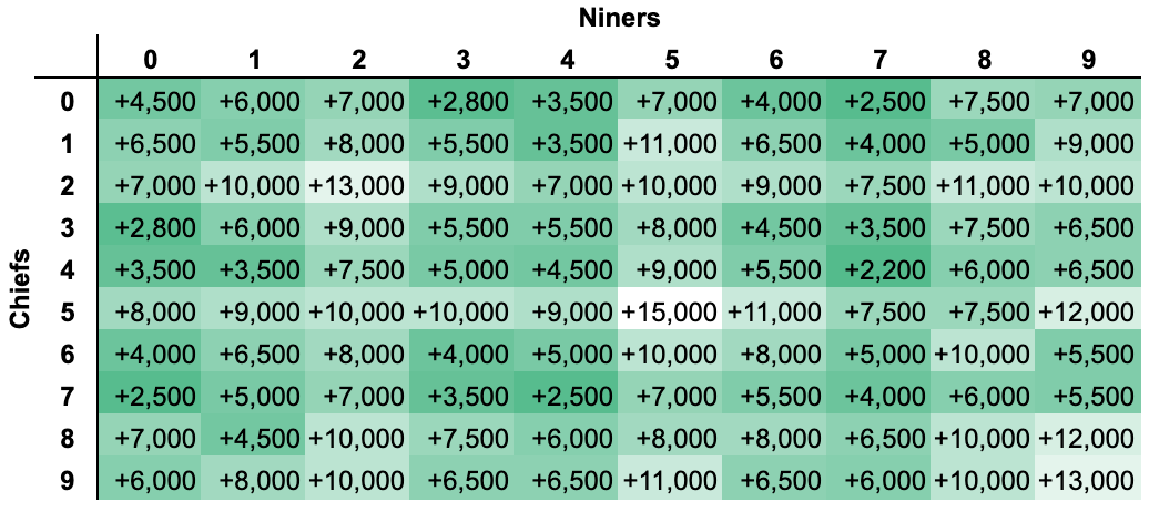
We then compared these frequencies with the publicly available betting odds offered on the ‘Super Bowl Squares – Final Result’ market by DraftKings Sportsbook to ascertain the expected value (EV) of each square
The analysis determined that all 100 of the available squares carried a negative expected value ranging from [-4.0% to -95.2%], and that buying all 100 squares would carry a negative expected value of approximately [-39.7%]
Our Methodology
We collected final game scores data from Pro Football Reference for the last 30 full NFL seasons, as well as the current NFL season through the completion of Week 17. We also included all Super Bowl games that took place prior to 30 seasons ago
Games that ended in a tie were excluded since that is not a potential outcome for the Super Bowl
We calculated raw frequencies for each of the 100 available squares, and then weighted the Niners’ digit 55% to the digit represented by the winner of the historical games, and 45% to the digit represented by the loser of the historical games. The [55% / 45%] weighting is reflective of the estimated win probability implied by the de-vigged Pinnacle Super Bowl Winner odds of ‘-129 / +117’ 23
The weighted frequencies were then multiplied by the gross payouts implied by DraftKings Sportsbook Super Bowl Squares – Final Result odds 2
Findings & Results
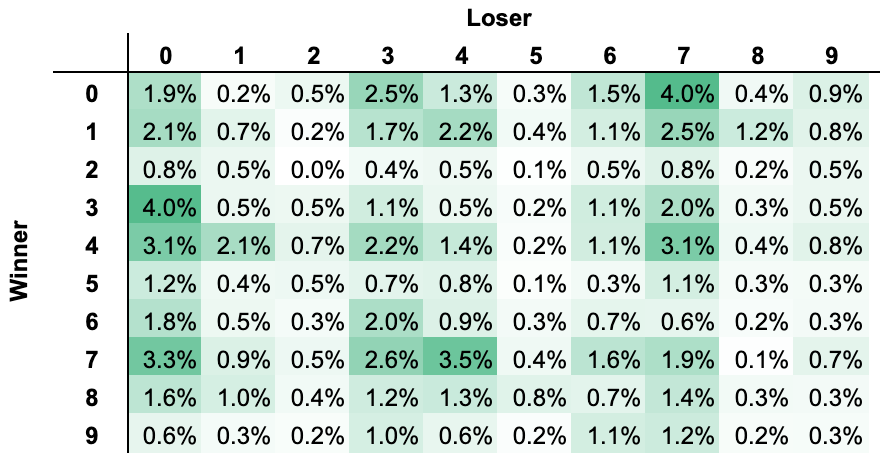
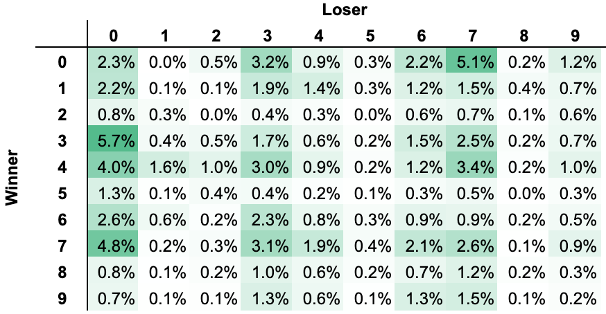
Raw Frequencies
Sample Size: n = 8,162 games
Most frequent digit for losing team is ‘0’, occurring ~20.5% of the time
Most frequent digit for winning team is ‘7’, occurring ~15.5% of the time
Losing Digit
Winning Digit
Frequency
7
0
3.99%
0
3
3.97%
4
7
3.47%
0
7
3.32%
0
4
3.11%
Top 5 most frequent winning squares
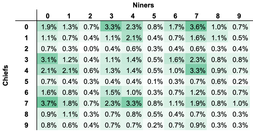
Weighted Frequencies
Sample Size: n = 8,162 games
Most frequent digit for Niners is ‘7’, occurring ~16.9% of the time
Most frequent digit for Chiefs is ‘0’, occurring ~17.4% of the time
Most frequent digit for losing team is ‘0’, occurring ~25.2% of the time
Most frequent digit for winning team is ‘4’, occurring ~16.3% of the time
Loser Digit
Winner Digit
Frequency
0
3
5.68%
7
0
5.09%
0
7
4.76%
0
4
3.98%
7
4
3.39%
Top 5 most frequent winning squares
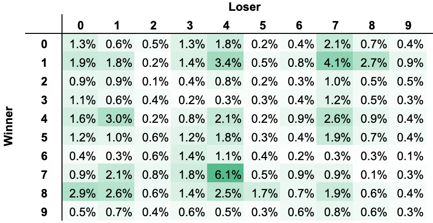
Raw Frequencies for Total Points o47.5
Sample Size: n = 3,035 games
Most frequent digit for losing team is ‘4’, occurring ~20.5% of the time
Most frequent digit for winning team is ‘1’, occurring ~17.9% of the time
Loser Digit
Winner Digit
Frequency
4
7
6.10%
7
1
4.09%
4
1
3.39%
1
4
2.97%
0
8
2.93%
Top 5 most frequent winning squares
Selected Conclusions
Participating in the “Super Bowl Squares – Final Result” market on DraftKings Sportsbook has a substantially negative overall expected value, and likely has a negative expected value for every single one of the 100 available squares
This conclusion is logically continuous with the fact that the probabilities implied by DraftKings’ available odds sum to a total of ~165.9%; the market has substantial “juice” or “vig” overall
The available odds on relatively common squares (e.g., [0:7], [3:0], [7:0]) are much closer to “fair” vs. the rarest square outcomes (e.g., [2:2], [5:5], [2:5])
This strategy by DraftKings entices bettors to place a substantial dollar volume of wagers on the “almost fair” squares that have a reasonable chance of winning
Secondarily, it mitigates the negative financial impact to DraftKings that could arise in the event of a “black swan” final game score, such as [15 – 5] or [22 – 12]
A participant who has a bias towards a “high-scoring” vs. “low-scoring” game would place materially different value on certain square outcomes. Amongst the most pronouncedly:
If one believes the game will be “low-scoring”, he should greatly value the losing team’s digit ‘0’, which occurs in 25.2% of low-scoring games in the dataset, but only in 12.7% of high-scoring games in the dataset
If one believes the game will be “high-scoring”, he should greatly value the winning team’s digit ‘1’, which occurs in 17.9% of high-scoring games in the dataset, but only in 9.8% of low-scoring games in the dataset
Areas for Research Expansion
The most substantial limitation in our analysis is that the square frequencies are derived solely from historical game logs, as opposed to a Monte Carlo simulation model of this year’s Super Bowl matchup
As such, an analyst of this data is forced to balance (i) choosing the subset of games that are most comparable to the game being predicted, and (ii) leaving a sufficiently large number of games in the dataset to mitigate the impact of outlier game results
The variant of Super Bowl Squares that we analyzed (“Final Result”) is one of several commonly played variants, each of which has its quirks that would impact the analysis. Perhaps the most common is the variant in which winning squares are determined by the digits in the score at the end of ANY quarter (as opposed to only at the end of the game)
Further analysis could yield interesting insights regarding how the value of a given square changes as the game progresses. As an example, say that a team scores a safety (worth two points) in the 1st quarter of the game. Which final square results would see the greatest increase in estimated probability? Which would see the greatest decrease? Are there any squares that would only be minimally impacted?
See ‘Appendix A’ for elaboration on the winning criteria for this variant. ↩︎
Pinnacle Super Bowl Winner odds and DraftKings Sportsbook Super Bowl Squares – Final Result odds were both updated as of approximately 9 PM EST on February 9, 2024. ↩︎
See ‘Appendix B’ for elaboration on the benefit and detailed methodology of weighting the raw square values relative to win probability. ↩︎
Pinnacle Super Bowl Winner odds and DraftKings Sportsbook Super Bowl Squares – Final Result odds were both updated as of approximately 9 PM EST on February 9, 2024. ↩︎
See ‘Appendix C’ for the DraftKings Sportsbook odds that were applied to each square in order to calculate expected value. Odds were updated as of approximately 9 PM EST on February 9, 2024. ↩︎
Parentheses reflect negative values. For example, “(5.42%)” would reflect a negative expected value of 5.42%. ↩︎
Appendix A: Winning Criteria
The variant of “Super Bowl Squares” that we analyzed is settled based on the final digit of each team’s score once the game has been completed
Both teams’ digits must match for a square to be deemed a winner. As such, there are 100 potential outcomes, and there will always be exactly 1 victorious square out of these 100 potential outcomes.
A partial set of the final scores that would result in victory for an entrant with the square “Chiefs 7 – Niners 3” are as follows:
Chiefs 7 / Niners 3
Chiefs 7 / Niners 13
Chiefs 7 / Niners 23
Chiefs 7 / Niners 33
Chiefs 17 / Niners 3
Chiefs 17 / Niners 13
Chiefs 17 / Niners 23
Chiefs 17 / Niners 33
Chiefs 27 / Niners 3
Chiefs 27 / Niners 13
Chiefs 27 / Niners 23
Chiefs 27 / Niners 33
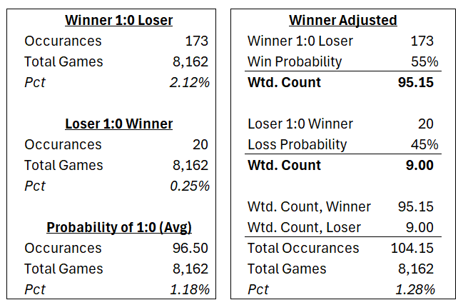
Appendix B: Weighted Square Value
Weighting is reflective of the estimated win probability implied by the de-vigged Pinnacle Super Bowl Winner odds of ‘-129 / +117’ [55% / 45% ]
Key Insight: If the winner is known, the square “Winner 1:0 Loser” increases from 1.2% to 2.2% probability, roughly doubling.
Scheduled Runs: You can set up automated dbt commands to run on a schedule, ensuring that your data modeling and transformation tasks are executed reliably and consistently.
Post-PR Merges: After merging a pull request into your project’s main branch, you have the option to trigger dbt runs. We recommend choosing either a full run or a state-aware run (which focuses only on modified models) to keep your project organized and efficient.
PR Commits Testing: To enhance your development process, dbt CI runs automatically on pull request commits. This helps you ensure that any changes you make are compatible and do not introduce unexpected issues into your data pipelines.
State Awareness: To utilize the state-aware workflow, it’s important to set up an S3 bucket to persist the manifest.json file. Additionally, Leveraging an S3 bucket to host the project documentation website, streamlines the documentation creation and adjustments within the development process.
Project and Environment Setup
1. Fork this repo and copy your whole dbt project into the project_goes_here folder. 2. Update your repository settings to allow GitHub Actions to create PRs. This setting can be found in a repository’s settings under Actions > General > Workflow permissions. It should look like this:
3. Go to the Actions tab and run the Project Setup workflow, making sure to select the type of database you want to set up – This opens a PR with our suggested changes to your profiles.yml and requirements.txt files. We assume if you’re migrating to self-hosting you need to add a prod target to your profiles.yml file, so this action will do that for you and also add the database driver indicated. 4. Add some environment variables to your GitHub Actions secrets in the Settings tab. You can see which vars are needed based on anything appended with ${{ secrets. in the open PR. Additionally, you need to define your AWS secrets to take advantage of state-aware builds – AWS_S3_BUCKET, AWS_ACCESS_KEY, & AWS_SECRET_KEY. 5. Run the Manual dbt Run to test that you’re good to go. 6. Edit the Actions you want to keep and delete the ones you don’t.
GitHub Actions Overview
Initially, we wanted to build out the project to a boilerplate CloudFormation stack that would create AWS resources to run a simple dbt core runner on EC2. We pivoted to using GitHub actions for cost and simplicity. GitHub gives you 2,000 free minutes of runner time. This works well for personal projects or organizations with sub-scale data, and if you need to scale beyond the free minutes, the cost is reasonable. Building with Github actions easily facilitates continuous integration, allowing you to automatically build and test data transformations whenever changes are pushed to the repository.
To cover most simple use cases we built some simple actions that run dbt in production to automate key aspects of your data pipeline.
Scheduled dbt Commands: You can set up scheduled dbt commands to run at specified intervals. This automation ensures that your data transformations are consistently executed, helping you keep your data up-to-date without manual intervention.
Pull Request Integration: After merging a pull request into the main branch of your repository, you can trigger dbt runs. This is a valuable feature for ensuring that your data transformations are validated and remain in a working state whenever changes are introduced. You have the flexibility to choose between a full run or a state-aware run, where only modified models are processed. This granularity allows you to balance efficiency with thorough testing.
dbt CI Runs: Pull requests often involve changes to your dbt models. To maintain data integrity, dbt CI checks are performed on pull request commits. This ensures that proposed changes won’t break existing functionality or introduce errors into your data transformations. It’s a critical step in the development process that promotes data quality.
State-Aware Workflow: The state-aware workflow requires an S3 bucket to store the manifest.json file. This file is essential for tracking the state of your dbt models, and by persisting it in an S3 bucket, you ensure that it remains available for reference and consistency across runs. Additionally, this S3 bucket serves a dual purpose by hosting your project’s documentation website, providing easy access to documentation related to your data transformations.
S3 Bucket and docs update
Hosting your dbt docs on S3 is a relatively simple and cost-effective way to make your documentation available. The process to generate the docs and push them to s3 happens during the “incremental dbt on merge”, “dbt on cron” jobs. The docs get generated by the “dbt docs generate” command and then are pushed to S3 by the upload_to_s3.py file. Adding this step to the workflow ensures the documentation is always current without much administrative complexity.
We added a CloudFormation template that creates an S3 bucket that is public facing as well as an IAM user that can get and push objects to the bucket. You will need to generate AWS keys for this user and add them to your project environment variables for it to work. If you are unfamiliar with CloudFormation we added some notes to the README.
quick note: the justification for doing this is worth like a 17 page manifesto. I’m focusing on the how, and maybe I’ll eventually write the manifesto.
General Approach
This specific problem is loading Point-of-Sale data for a vertical specific system into a database for analysis on a daily basis, but could be generalized to most small/medium data use cases where ~24 hour latency is totally fine.
The ELT pipeline uses Hex Notebooks and dbt jobs, both orchestrated independently with crons. dbt is responsible for creating all tables and handling grants as well as data transformation, while Hex handles extract and load from a set of REST APIs into the database. Hex loads into a “queue” of sorts – simply a table in Snowflake that can take JSON pages and some metadata. Conceptually, it looks like this.
Loading data with Hex
Since Hex is a python notebook running inside of managed infrastructure, we can skip the nonsense of environment management, VMs, orchestration, and so on and just get to loading data. First things first, lets add the snowflake connector to our environment.
Bash
!pip3installsnowflake-connector-python
Now that we have added that package our environment, we can build our python functions. I’ve added some simple documentation below.
Python
import requestsimport osimport jsonimport snowflake.connectorfrom snowflake.connector.errors import ProgrammingErrorfrom datetime import datetime# login to snowflakedefsnowflake_login(): connection = snowflake.connector.connect(user=SNOWFLAKE_USER,password=SNOWFLAKE_PASSWORD,account=SNOWFLAKE_ACCOUNT,database=os.getenv('SNOWFLAKE_DATABASE'),schema=os.getenv('SNOWFLAKE_SCHEMA'),warehouse=os.getenv('SNOWFLAKE_WAREHOUSE'), )# print the database and schemaprint(f"Connected to database '{os.getenv('SNOWFLAKE_DATABASE')}' and schema '{os.getenv('SNOWFLAKE_SCHEMA')}'")return connection# get the last run date for a specific endpoint and store from snowflakedeflast_run_date(conn, table_name, store_name): cur = conn.cursor()try:# Endpoints take UTC time zoneprint(f"SELECT MAX(UPDATED_AT) FROM PROD_PREP.{table_name} WHERE store_name = '{store_name}';") query = f"SELECT MAX(UPDATED_AT) FROM PROD_PREP.{table_name} WHERE store_name = '{store_name}'" cur.execute(query) result = cur.fetchone()[0]try: result_date = datetime.strptime(str(result).strip("(),'"), '%Y-%m-%d %H:%M:%S').date()exceptValueError:# handle the case when result is None or not in the expected formattry: result_date = datetime.strptime(str(result).strip("(),'"), '%Y-%m-%d %H:%M:%S.%f').date()exceptValueError:print(f"error: Cannot handle datetime format. Triggering full refresh.") result_date = '1900-01-01'except ProgrammingError as e:if e.errno == 2003:print(f'error: Table {table_name} does not exist in Snowflake. Triggering full refresh.')# this will trigger a full refresh if there is an error, so be careful here result_date = '1900-01-01'else:raise e cur.close() conn.close()return result_date# Request pages, only return total page numberdefget_num_pages(api_endpoint,auth_token,as_of_date): header = {'Authorization': auth_token} total_pages = requests.get(api_endpoint+'?page=1&q[updated_at_gt]='+str(as_of_date),headers=header).json()['total_pages']return total_pages# Returns a specific page given a specific "as of" date and page numberdefget_page(api_endpoint,auth_token,as_of_date,page_num): header = {'Authorization': auth_token}print(f"loading data from endpoint: {api_endpoint}" ) page = requests.get(api_endpoint+'?page='+str(page_num)+'&q[updated_at_gt]='+str(as_of_date),headers=header).json()return page# Loads data into snowflakedefload_to_snowflake(store_name, source_api, api_key, updated_date, total_pages, conn, stage_table, json_element): cur = conn.cursor() create_query = f"CREATE TABLE IF NOT EXISTS {stage_table} ( store_name VARCHAR , elt_date TIMESTAMPTZ, data VARIANT)" cur.execute(create_query)# loop through the pagesfor page_number inrange(1,total_pages+1,1): response_json = get_page(source_api,api_key,updated_date,page_number) raw_json = response_json[json_element] raw_data = json.dumps(raw_json)# some fields need to be escaped for single quotes clean_data = raw_data.replace('\\', '\\\\').replace("'", "\\'") cur.execute(f"INSERT INTO {stage_table} (store_name, elt_date, data) SELECT '{store_name}', CURRENT_TIMESTAMP , PARSE_JSON('{clean_data}')")print(f"loaded {page_number} of {total_pages}") cur.close() conn.close()# create a wrapper for previous functions so we can invoke a single statement for a given APIdefjob_wrapper(store_name, api_path, api_key, target_table, target_table_key):# get the updated date for a specific table updated_date = last_run_date(snowflake_login(), target_table, store_name)print(f"The maximum value in the 'updated_at' column of the {target_table} table is: {updated_date}")# get the number of pages based on the updated date pages = get_num_pages(api_path,api_key,updated_date)print(f"There are {pages} pages to load in the sales API")# load to snowflake load_to_snowflake(store_name, api_path, api_key,updated_date,pages,snowflake_login(),target_table, target_table_key)
Now that we have our python in place, we can invoke a specific API. It should be noted that Hex also has built-in environmental variable management, so we can keep our keys safe while still having a nice development & production flow.
To deploy this for more endpoints, simply update the api_url, end_point_name, and endpoint_unique_id. You can also hold it in a python dict and reference it as a variable, but I found that to be annoying when troubleshooting.
The last step in Hex is to publish the notebook so that you can set a cron job on it – I set mine to run at midnight PST.
Transforming in dbt
I am using on-run-start & on-run-end scripts in my dbt project to frame out the database, in my case, Snowflake.
SQL
on-run-start: - CREATETABLEIFNOTEXISTS STAGING.sales_histories ( store_name VARCHAR , elt_date TIMESTAMPTZ, data VARIANT, id INT) ;
Now that data is in snowflake (in the RAW schema), we can use a macro in dbt to handle our transformation from pages coming from the API to rows in a database. But first we need to define our sources (the tables built in the on-run-start step) in YAML.
Of course, the real magic here is in the “merge_queues” macro, which is below:
SQL
{% macro merge_queues( table_name, schema, unique_id )%}MERGEINTO {{schema}}.{{table_name}} tUSING (with cte_top_level as (-- we can get some duplicate records when transaction happen as the API runs-- as a result, we want to take the latest date in the elt_date column-- this used to be a group by, and now is qualifyselect store_name, elt_date,valueas val, val:{{unique_id}} as idfromRAW.{{table_name}}, lateral flatten( input => data ) QUALIFY ROW_NUMBER() OVER (PARTITIONBY store_name, id ORDER BY elt_date desc) = 1 )select *from cte_top_level ) sON t.id = s.id AND t.store_name = s.store_name-- need to handle updates if they come inWHENMATCHEDTHENUPDATESET t.store_name = s.store_name, t.elt_date = s.elt_date, t.data = s.val, t.id = s.idWHENNOTMATCHEDTHENINSERT ( store_name, elt_date, data, id)VALUES ( s.store_name, s.elt_date, s.val, s.id);-- truncate the queueTRUNCATERAW.{{table_name}};{% endmacro %}
A key note here is that snowflake does not handle MERGE like an OLTP database, so we need to de-duplicate it before we INSERT or UPDATE. I learned this the hard way by trying to de-dupe once the data was into my staging table, but annoyingly this is not easy in snowflake! So I had to truncate and try again a few times.
Now that the data is in a nice tabular format, we can run it like a typical dbt project.
Let me know if you have any questions or comments – you can find me on twitter @matsonj
Other notes
There are lots of neat features that I didn’t end up implementing. A noncomprehensive list is below:
Source control + CI/CD for the Hex notebooks – the Hex flow is so simple that I didn’t feel this was necessary.
Hex components to reduce repetition of code – today, every store gets its own notebook.
Using mdsinabox patterns with DuckDB instead of Snowflake – although part of the reason to do this was to defer infrastructure to bundled vendors.
I didn’t really set out to learn Docker when I started the MDS-in-a-box project, but as it turns out, Docker is quite a good fit. Part of this is because I desired to run the project in a Github Action, which is a very similar paradigm, and also because I have the notion (TBD) of running a bunch of simulations in AWS Batch. The goal of this post is to show a quick demo and then summarize what I learned – which frankly will also serve as a quick reference for me when I use Docker again.
Running the project in Docker
Once Docker Desktop is installed, building the project is trivial with two ‘make’ scripts.
make docker-build
make docker-run-superset
This takes a few minutes, but once its complete you have a full operational analytics stack running inside your machine.
The first rule of Docker
I learned this one the hard way, as I attempted to add evidence.dev to my existing container. The environment was only based on Python, and I needed to add Node support to it. I tried and tried to modify the dockerfile to get Node working – which leads to the first rule of Docker:
Thou Shalt Use An Existing Base Image
As it turns out, a quick googling revealed that there was already an awesome set of python+node base images. Shout out to this repo which is what I ended up using: Python with Node.js.
Now that I had the Docker container “working” – I needed to actually figure out which docker commands to use.
Docker Quick Reference
These are the commands that I learned and used over and over again as I triaged my way through adding another component to my environment. It is not exhaustive but designed to be a practical list of key commands to help you get started with Docker, too.
docker build – use this to build the image defined in your working directory. In my project, I’m also giving it a name (-t mdsbox) and defining where to save it, so the full command is ‘docker build -t mdsbox .‘
docker run – use this to run your image as a container once its built. You also pass in your environmental variables as part of docker run, so this command gets a bit long. Unfortunately, this is the first command that you see when learning Docker, which makes it look more imposing and scary than it actually is. The general syntax is ‘docker run <docker config> <CLI command>‘.
docker ps – use this command to see which containers are running. This is so you know which containers to stop or to access (via docker exec) within the CLI.
docker stop – this command stops a container. If you run a container from the terminal, you can’t stop it or exit like a process running in the terminal (i.e. with Ctrl+D), so you need to use ‘docker stop <container name>‘ instead!
docker exec – this command lets you run a command on a running container. I found this be absolutely huge for debugging as you can get right into the terminal on your container and futz around with it. The command I used to access it is ‘docker exec -it <container name> /bin/bash‘ which drops you into the terminal.
–publish – I’m including this Docker flag, since this is the flag you invoke to make your application visible on the network. Used in context, it looks something like this: ‘docker run –publish 3000:3000 <container name>‘. It is simply mapping port 3000 on the host to port 3000 on the container.
There are some notable exclusions, like ‘docker pull‘ but this reference is merely to help get started with MDS-in-a-box. By the way, you can check out the latest deployed version at www.mdsinabox.com!
As a note, I want to thank Pedram Navid & Greg Wilson for being my Docker shepherds – I definitely was stuck a few times and your guidance was incredibly helpful in getting things unstuck!
TLDR: A fast, free, and open-source Modern Data Stack (MDS) can now be fully deployed on your laptop or to a single machine using the combination of DuckDB, Meltano, dbt, and Apache Superset.
This post is a collaboration with Jacob Matson and cross-posted on DuckDB.org.
Summary
There is a large volume of literature (1, 2, 3) about scaling data pipelines. “Use Kafka! Build a lake house! Don’t build a lake house, use Snowflake! Don’t use Snowflake, use XYZ!” However, with advances in hardware and the rapid maturation of data software, there is a simpler approach. This article will light up the path to highly performant single node analytics with an MDS-in-a-box open source stack: Meltano, DuckDB, dbt, & Apache Superset on Windows using Windows Subsystem for Linux (WSL). There are many options within the MDS, so if you are using another stack to build an MDS-in-a-box, please share it with the community on the DuckDB Twitter, GitHub, or Discord, or the dbt slack! Or just stop by for a friendly debate about our choice of tools!
Motivation
What is the Modern Data Stack, and why use it? The MDS can mean many things (see examples here and a historical perspective here), but fundamentally it is a return to using SQL for data transformations by combining multiple best-in-class software tools to form a stack. A typical stack would include (at least!) a tool to extract data from sources and load it into a data warehouse, dbt to transform and analyze that data in the warehouse, and a business intelligence tool. The MDS leverages the accessibility of SQL in combination with software development best practices like git to enable analysts to scale their impact across their companies.
Why build a bundled Modern Data Stack on a single machine, rather than on multiple machines and on a data warehouse? There are many advantages!
Simplify for higher developer productivity
Reduce costs by removing the data warehouse
Deploy with ease either locally, on-premise, in the cloud, or all 3
Eliminate software expenses with a fully free and open-source stack
Maintain high performance with modern software like DuckDB and increasingly powerful single-node compute instances
Achieve self-sufficiency by completing an end-to-end proof of concept on your laptop
Enable development best practices by integrating with GitHub
Enhance security by (optionally) running entirely locally or on-premise
If you contribute to an open-source community or provide a product within the Modern Data Stack, there is an additional benefit!
Increase adoption of your tool by providing a free and self-contained example stack
Reach out on the DuckDB Twitter, GitHub, or Discord, or the dbt slack to share an example using your tool with the community!
Trade-offs
One key component of the MDS is the unlimited scalability of compute. How does that align with the MDS-in-a-box approach? Today, cloud computing instances can vertically scale significantly more than in the past (for example, 224 cores and 24 TB of RAM on AWS!). Laptops are more powerful than ever. Now that new OLAP tools like DuckDB can take better advantage of that compute, horizontal scaling is no longer necessary for many analyses! Also, this MDS-in-a-box can be duplicated with ease to as many boxes as needed if partitioned by data subject area. So, while infinite compute is sacrificed, significant scale is still easily achievable.
Due to this tradeoff, this approach is more of an “Open Source Analytics Stack in a box” than a traditional MDS. It sacrifices infinite scale for significant simplification and the other benefits above.
Choosing a problem
Given that the NBA season is starting soon, a monte carlo type simulation of the season is both topical and well-suited for analytical SQL. This is a particularly great scenario to test the limits of DuckDB because it only requires simple inputs and easily scales out to massive numbers of records. This entire project is held in a GitHub repo, which you can find here: https://www.github.com/matsonj/nba-monte-carlo.
Building the environment
The detailed steps to build the project can be found in the repo, but the high-level steps will be repeated here. As a note, Windows Subsystem for Linux (WSL) was chosen to support Apache Superset, but the other components of this stack can run directly on any operating system. Thankfully, using Linux on Windows has become very straightforward.
Install Ubuntu 20.04 on WSL.
Upgrade your packages (sudo apt update).
Install python.
Clone the git repo.
Run make build and then make run in the terminal.
Create super admin user for Superset in the terminal, then login and configure the database.
Run test queries in superset to check your work.
Meltano as a wrapper for pipeline plugins
In this example, Meltano pulls together multiple bits and pieces to allow the pipeline to be run with a single statement. The first part is the tap (extractor) which is ‘tap-spreadsheets-anywhere‘. This tap allows us to get flat data files from various sources. It should be noted that DuckDB can consume directly from flat files (locally and over the network), or SQLite and PostgreSQL databases. However, this tap was chosen to provide a clear example of getting static data into your database that can easily be configured in the meltano.yml file. Meltano also becomes more beneficial as the complexity of your data sources increases.
plugins:
  extractors:
  - name: tap-spreadsheets-anywhere
    variant: ets
    pip_url: git+https://github.com/ets/tap-spreadsheets-anywhere.git
# data sources are configured inside of this extractor
The next bit is the target (loader), ‘target-duckdb‘. This target can take data from any Meltano tap and load it into DuckDB. Part of the beauty of this approach is that you don’t have to mess with all the extra complexity that comes with a typical database. DuckDB can be dropped in and is ready to go with zero configuration or ongoing maintenance. Furthermore, because the components and the data are co-located, networking is not a consideration and further reduces complexity.
Next is the transformer: ‘dbt-duckdb‘. dbt enables transformations using a combination of SQL and Jinja templating for approachable SQL-based analytics engineering. The dbt adapter for DuckDB now supports parallel execution across threads, which makes the MDS-in-a-box run even faster. Since the bulk of the work is happening inside of dbt, this portion will be described in detail later in the post.
Lastly, Apache Superset is included as a Meltano utility to enable some data querying and visualization. Superset leverages DuckDB’s SQLAlchemy driver, duckdb_engine, so it can query DuckDB directly as well.
With Superset, the engine needs to be configured to open DuckDB in “read-only” mode. Otherwise, only one query can run at a time (simultaneous queries will cause locks). This also prevents refreshing the Superset dashboard while the pipeline is running. In this case, the pipeline runs in under 8 seconds!
Wrangling the data
The NBA schedule was downloaded from basketball-reference.com, and the Draft Kings win totals from Sept 27th were used for win totals. The schedule and win totals make up the entirety of the data required as inputs for this project. Once converted into CSV format, they were uploaded to the GitHub project, and the meltano.yml file was updated to reference the file locations.
Loading sources
Once the data is on the web inside of GitHub, Meltano can pull a copy down into DuckDB. With the command meltano run tap-spreadsheets-anywhere target-duckdb, the data is loaded into DuckDB, and ready for transformation inside of dbt.
Building dbt models
After the sources are loaded, the data is transformed with dbt. First, the source models are created as well as the scenario generator. Then the random numbers for that simulation run are generated – it should be noted that the random numbers are recorded as a table, not a view, in order to allow subsequent re-runs of the downstream models with the graph operators for troubleshooting purposes (i.e. dbt run -s random_num_gen+). Once the underlying data is laid out, the simulation begins, first by simulating the regular season, then the play-in games, and lastly the playoffs. Since each round of games has a dependency on the previous round, parallelization is limited in this model, which is reflected in the dbt DAG, in this case conveniently hosted on GitHub Pages.
There are a few more design choices worth calling out:
Simulation tables and summary tables were split into separate models for ease of use / transparency. So each round of the simulation has a sim model and an end model – this allows visibility into the correct parameters (conference, team, elo rating) to be passed into each subsequent round.
To prevent overly deep queries, ‘reg_season_end’ and ‘playoff_sim_r1’ have been materialized as tables. While it is slightly slower on build, the performance gains when querying summary tables (i.e. ‘season_summary’) are more than worth the slowdown. However, it should be noted that even for only 10k sims, the database takes up about 150MB in disk space. Running at 100k simulations easily expands it to a few GB.
Connecting Superset
Once the dbt models are built, the data visualization can begin. An admin user must be created in superset in order to log in. The instructions for connecting the database can be found in the GitHub project, as well as a note on how to connect it in ‘read only mode’.
There are 2 models designed for analysis, although any number of them can be used. ‘season_summary’ contains various summary statistics for the season, and ‘reg_season_sim’ contains all simulated game results. This second data set produces an interesting histogram chart. In order to build data visualizations in superset, the dataset must be defined first, the chart built, and lastly, the chart assigned to a dashboard.
Below is an example Superset dashboard containing several charts based on this data. Superset is able to clearly summarize the data as well as display the level of variability within the monte carlo simulation. The duckdb_engine queries can be refreshed quickly when new simulations are run.
season summary & expected winsplayoff results
Conclusions
The ecosystem around DuckDB has grown such that it integrates well with the Modern Data Stack. The MDS-in-a-box is a viable approach for smaller data projects, and would work especially well for read-heavy analytics. There were a few other learnings from this experiment. Superset dashboards are easy to construct, but they are not scriptable and must be built in the GUI (the paid hosted version, Preset, does support exporting as YAML). Also, while you can do monte carlo analysis in SQL, it may be easier to do in another language. However, this shows how far you can stretch the capabilities of SQL!
Next steps
There are additional directions to take this project. One next step could be to Dockerize this workflow for even easier deployments. If you want to put together a Docker example, please reach out! Another adjustment to the approach could be to land the final outputs in parquet files, and to read them with in-memory DuckDB connections. Those files could even be landed in an S3-compatible object store (and still read by DuckDB), although that adds complexity compared with the in-a-box approach! Additional MDS components could also be integrated for data quality monitoring, lineage tracking, etc.
Josh Wills is also in the process of making an interesting enhancement to dbt-duckdb! Using the sqlglot library, dbt-duckdb would be able to automatically transpile dbt models written using the SQL dialect of other databases (including Snowflake and BigQuery) to DuckDB. Imagine if you could test out your queries locally before pushing to production… Join the DuckDB channel of the dbt slack to discuss the possibilities!
Please reach out if you use this or another approach to build an MDS-in-a-box! Also, if you are interested in writing a guest post for the DuckDB blog, please reach out on Discord!